Week 1 Project Ideas

Project 1: Respiratory central pattern generator network in mammalian brainstem (Rubin et al. 2009)

Stereotypical rhythmic behaviours, both voluntary and involuntary, locomotion and breathing are generated by CPGs (Central Pattern Generators). These patterns are generated by interactions betweens the group of neurons (Nuclei or ganglion). Some special networks of these nuclei are capable of generating endogenous rhythms. These do not require rhythmic inputs but inherently generate patterned rhythmic patterns. Rubin et al 2009 models one such respiratory CPG located in the lower brain stem of mammalian brain. The motor pattern observed during normal breathing is considered to consist of three phases: a phase of inspiration, associated with phrenic motor activity producing lung inflation, and two expiratory phases: post-inspiration and late (stage 2) expiration. The simple things you can demonstrate with this model readily are :

(a) This tri-phasic response is shifted to a bi-phasic response when inputs from pons are removed.

(b) When more caudal inputs are reduced, the response shifts to a mono-phasic response.

(c) If you can control INap somehow (optogenetically or using blockers), it does not cause shift in the phase but changes its period.

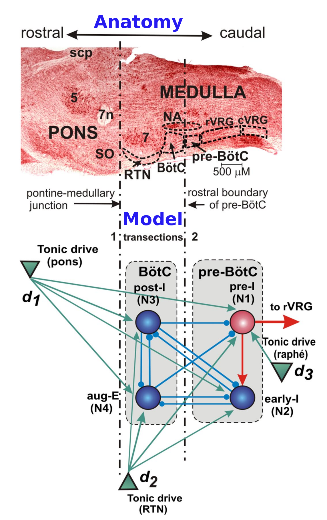
Citation-Multiple rhythmic states in a model of the respiratory central pattern generator doi:10.1152/jn.90958.2008

You can do many more things with this model. Abovementioned suggestions are just characterizations of the model. Some suggestions are as follows :

Bifurcation diagrams drawn using different bifurcation parameters can give you more clues about possibilities you can explore with this model. For example : You can investigate how more realistic patterns can be generated from controlling the drive to the CPGs. Let’s say you look at a paper like this. This measures complex-realistic breathing rhythms in mice. What are the ways to generate this kind of rhythm ? Are some inputs here voluntary (controlled by cerebral cortex) and involuntary ? (brainstem-intrinsic drive). How the breathing patterns are in behaviours where voluntary drive is extreme (high-singing, low or zero-sleeping/anesthesia) .

Project 2: Inverse stochastic resonance in Purkinje cells of cerebellum and its functional role in locally optimal information transfer (Buchin et al., 2016)

XPPAUT/MATLAB Code link

Purkinje neurons perform prominent computations in cerebellum through long dendritic arbours that go deep into cerebellar structures, unlike any other neuron type present in cerebellum. They have been shown to exhibit complex dynamics, display bistability and also display many interesting network phenomena like high frequency oscillations and travelling waves. Another special feature of these neurons is that they possess an excitability mechanism that allows them to be efficiently inhibited by a noise of a particular range of variance. This phenomenon is known as inverse stochastic resonance or ISR (for more details about this special phenomena and its other counterpart, ie, stochastic resonance refer to this) . Buchin et al 2016 present a simplified model of Purkinje neurons (adLIF experimentally fitted to purkinje neurons) . They and others have shown that a dynamical system with bistability is much needed to display ISR. What is interesting is that ISR allows purkinje neurons to efficiently perform many computations by operating in many regimes: ON and OFF (all-or-none toggle) or a filtering regime. Synaptic noise, or the noisy nature of synaptic firing (which we now know to be a feature and not a bug) allows purkinje cells to switch between these functional regimes. In essence, authors provide first evidence of functional significance of ISR . You can start with following things:

(a) Characterize the purkinje neuron wrt its excitability type, ie. type I or type II based on its Freq-Response curve. This gives us some clues about its dynamics. Compare the result of a ramping current input to your simulated neurons to an experimentally measured purkinje cell recording.

(b) The adLIF neuron was first formally described by Brete and Gerstner in 2003. Have a quick glimpse of their original paper and figure out which parameters control what aspect of the cell’s firing ? (adaptation, excitability type etc)

(c) Demonstrate that the Purkinje cells (simulated) show ISR for a particular variance band. How big is this band ? What parameters of the noise are important (mean,variance,duration etc) ? Does it matter what the distribution of the noise is ? (gaussian, poissonian,uniform, etc )

(d) Draw the bifurcation plot of the Purkinje neuron using XPPAUT. For what values of Iapp do you observe a Hopf bifurcation?

(e) Is there any relation between the values of variance for which the neuron shows ISR and where it shows the bifurcation ? Basically how is ISR related to the dynamics of the cell ?

(f) Something interesting I can suggest is as follows : change some intrinsic parameter, i.e., lets say adaptation rate or leak reversal or delta, a ,b. This now is not purkinje neuron anymore. Now redraw the bifurcation plot and again do (e). Where do the phenomena of ISR break down/modified/changed/become less stringent ?

(g) adLIF or Gerstner’s adLIF can exhibit both type I and type II excitability. Type I excitability: Neurons can fire at arbitrarily low frequencies just above threshold. Associated with a saddle-node bifurcation on an invariant circle (SNIC).Type II excitability: Neurons start firing at a finite frequency once threshold is crossed. Associated with a Hopf bifurcation. Now you must have characterized your neuron in (a). Does the other type exhibit ISR ? Why or why not ? (some hints might be in the bifurcation plot).

You can do many more things with this model. Abovementioned suggestions are just characterizations of the model. Some interesting broad questions to ask might be :

How ISR transforms short and long inputs in presence and absence of noise? What kind of computation does noise help with? Etc. . Another important thing to remember is : The function of cerebellar Purkinje cells is often considered in the context of adaptive filter models of the cerebellum.

Project 3: Binocular rivalry in a simple two-neuron model

(Original Source-link)

In binocular rivalry each eye views a different image but our perception alternates (time scale of seconds) between the images. Several existing models account for the oscillations by incorporating two neuronal populations that compete through mutual inhibition. A slow fatiguing mechanism, such as adaptation, mediates the back and forth switching of dominance. Here we study a simple ring-rate model. Let uj(t) be the ring rate of population j (j = 1, 2); aj(t) are the slow adaptation variables. The firing rates of the populations evolve in time according to the following set of ODEs:

duj/dt = -uj + f(-βui -γaj + Ij)

daj/dt = (uj -aj)/τa

with f(x) = 1/(1 + exp((θ − x)/k) and control parameter values: β = 0.9, γ = 0.5, I1= I2 = 0, τa = 10, θ = 0.2, k = 0.1.

1. Identify and describe the terms and parameters in the model (inhibition, external input, etc.)

2. Show that for β = 0.9 and I = 0.8 the model oscillates. Plot the time courses of u₁ and a₁ on the same axes (ordinate: -0.1 to 1.1, abscissa: 0 to 300), and describe the behavior (phases of dominance, suppression, etc). Overlay u₁ and u₂ on another plot and describe the trajectory. The underlying mechanism is bistability in the fast dynamics. Show it: think of a_j as slow; freeze them, say at 0.5 and look at u₁ and u₂ -nullclines.

3. Show that the model oscillates for a range of I -values; compute and plot the period, T vs I ; also plot max and min of u₁ vs I . According to Levelt’s Proposition 1 (LP1), based on psychophysical experiments, the oscillation period is expected to decrease as I increases. Does the model satisfy LP1?

4. Increase β (to 1.1) and compute the model’s behavior for 0 < I < 2.5; summarize it in a plot of amplitude vs I (bifurcation diagram); also, T vs I . Note and describe the new behavior (Winner-Take-All, WTA) for an intermediate range of I . Use some phase plane projections to demonstrate bistability in this WTA regime. For what I-range(s) is LP1 (more-or-less) satisfied or not satisfied?

5. Show that decreasing τₐ eliminates oscillations (why?) and leaves only the WTA regime.

6. Complete your response diagrams of amplitude of u₁ vs I by including the special uniform steady state (time independent, u₁ = u₂ , a₁ = a₂ ). Can you show analytically that it is monotonic?

7. Identify the kinds of bifurcations that occur as different solution states appear/disappear.

Project 4: Persistent spiking as a potential mechanism for supporting working memory (Ratte et al., 2018)

Github Repository

Most of the neurons use spikes to encode information. Some neurons can store information for short periods (seconds to minutes) by continuing to spike even after the stimulus is over. This mechanism has been speculated as a potential mechanism to enable working memory. This so-called “persistent” spiking occurs in many brain areas like medial prefrontal cortex (PFC),anterior cingulate cortex (ACC),Hippocampus,Amygdala and Entorhinal Cortex (EC). For example: Neurons of the prefrontal cortex exhibit persistent firing during the delay period of working memory tasks (Galloway, Evan M et al.). There is strong experimental evidence in PFC that Acetylcholine receptors (Muscarinic receptor) blockade compromises both working memory and persistent spiking activity. There are many possible mechanisms suggested for persistent spiking, recurrent connections and intrinsic neuronal bistability are a few to name. Intrinsic bistability has been linked to the calcium-activated, nonspecific cation current (ICAN), which has in turn, been linked to canonical transient receptor potential (TRPC) channels, especially TRPC5. These channels are gated by an influx of calcium.

Ratte et al. 2018 constructed a detailed model for ACC pyramidal neuron.

The simple things you can demonstrate with this model readily are :

a. Show that the ACC neurons show persistent firing even after the stimulus is off. Confirm whether it switches off the persistent firing after a long time ? If not, how can you switch off the persistent firing ?

b. You can draw the F-I curve of this neuron for different values of calcium activated nonspecific current (ICAN). See if this leads you to some interesting place ?

c. Use XPPAUT to draw a bifurcation plot for this neuron. You can choose different bifurcation parameters, depending upon what you find useful from the paper. What bifurcation does the system undergo and for what values of the bifurcation parameter?

You can do many more things with this model. Abovementioned suggestions are just characterizations of the model. Some interesting broad questions to ask might be :

You can do many things here. For example : look at this cartoon (link)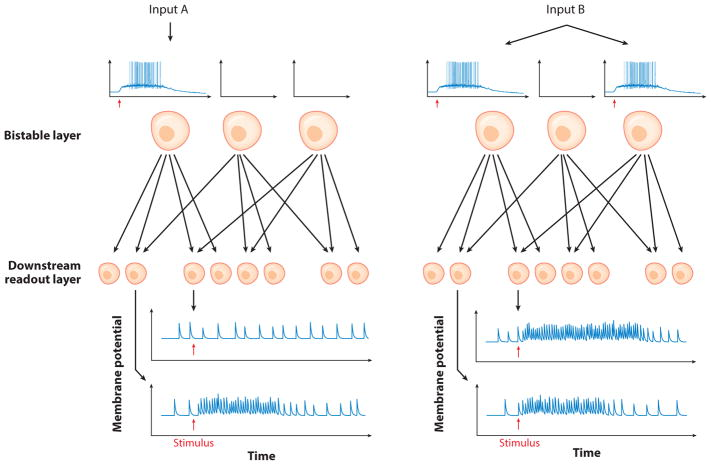

This cartoon is a simplified version of how a feed forward layer of bistable neurons that show persistent firing, can be used as a model to encode memory of a stimulus for a short time, even after the stimulus is gone. You can go this route or think of something more creative as well. What is the information content of stimulus in persistent firing ? You might have to look at the output of a group of ACC neurons.

Project 5: On simple connectivity structure to generate oscillations

Objective:

This project explores how simple rules on the structure of connectivity can explain the emergence of oscillations. Starting with a simple linear system, one can derive a very simple rule due to Thomas [1]: if the number of inhibitory connections of the loops present in a linear network is odd, then oscillation will possibly emerge. This was proved by Snoussi [2] and Gouzé [3]. In a simple non-linear neural system, the threshold-linear model, there are some additional constraints on the weights [4].

1. The emergence of oscillations in linear systems:

The presence of oscillations can be determined by analysing the spectral properties of the Jacobian matrix of dynamical systems. Familiarising with this concept can be done through simple analytical computations as well as simulations.

2. Going beyond linearity:

The conditions for oscillations proposed in [4] for threshold-linear model can be tested numerically. What happens in more general networks with several loops as well as in spiking networks are very interesting open questions.

Outcome: Learn how fundamental connectivity rules (like inhibitory loops and excitation-inhibition balance) generate neural oscillations. By combining theory with simulations, students gain intuition for how network structure shapes dynamics — a key concept for understanding rhythms in biological and artificial neural circuits. The hands-on analysis reinforces how mathematical principles translate to observable phenomena in neuroscience.

References:

[1] Thomas R. 1980. On the relation between the logical structure of systems and their ability to generate multiple steady States or sustained Oscillations. Thomas R (Ed). Numerical Methods in the Study of Critical Phenomena. Springer. p. 180—193.

[2] Snoussi EH. 1998. Necessary conditions for multistationarity and stable periodicity. Journal of Biological Systems 06:3--9

[3] Gouzé JL. 1998. Positive and negative circuits in dynamical systems. Journal of Biological Systems 06:11--15.

[4] Zang, J., Liu, S., Helson, P. & Kumar, A. Structural constraints on the emergence of oscillations in multi-population neural networks. eLife 12, RP88777 (2024).

Project 6: Graded persistent activity in the pre-frontal cortex

The persistent activity in the cortex is a phenomenon where the firing of a neuron or neural circuit that exceeds the duration of a stimulus, persisting after the stimulus has terminated. This has been shown to be important for the generation of functions such as working memory in the cortex. Here we will study how single neuron in the prefrontal cortex.

Implement the pre-frontal cortex conductance based model as described in Hyperpolarization- activated graded persistent activity in the prefrontal cortex (https://doi.org/10.1073/pnas.0800360105). Or you can find other models of single-neuron persistent activity.

As the paper points out, the Ih current is essential for developing the graded activity of the neurons. What other factors of the model and the different ion channels affect graded activity and how?
How does the dynamics of the different ion channels play out in the model? Use appropriate values of different currents and see large-scale realtion between them.

Project 7: Spike filtering with short-term plasticity

Short-term plasticity is responsible for facilitating/depressing synapses at very short timescales of the order of 10s of ms. It is believed to play an important role in neuronal computation by providing a form of rate-filtering mechanism.

Develop a simple short-term plasticity model like in:

a. (Tsodyks M, Pawelzik K, Markram H. 1998): Neural networks with dynamic synapses

(https://doi.org/10.1162/089976698300017502)

b. (Lee et al. 2009): A Kinetic Model Unifying Presynaptic Short-Term Facilitation and Depression (https://doi.org/10.1007/s10827-008-0122-6)

Explore the different kinds of synapses (facilitating and depressing) by changing the parameters to get the behaviour of different kinds of synaptic connections in the brain.

How would you change the parameters to get different ranges of rate filtering (eg. 10- 30Hz)?
Look at how the filtering mechanism behaves of the stimulus is changed to a Poisson train of the same rate/frequency instead of a regular periodic stimulus
What are the limits of this system?

Project 8: Pyramidal neurons in CA1 switch from integrators to resonators (Prescott et al. 2008) :

Github Repository

When the animal is in an active state (wakefulness) , pyramidal neurons typically experience a lot of synaptic inputs that causes tonic depolarisation, causes the resting membrane potential to rise (shunting) and noisy fluctuations. In contrast, pyramidal neurons in slices do not experience such a big barrage of synaptic inputs. Prescott et al 2008 claims that due to this discrepancy between in-vitro and and in-vivo conditions, the preposition that pyramidal neurons that are usually characterized as class 1 ( integrators ) is not that accurate. Conversely, the animal can have different states of inputs gathered at CA1 depending upon task and attention levels. They show that CA1 pyramidal neurons can transition from Integrator to resonator based on shunting levels and levels of adaptation Mechanistically, shunting and adaptation can change spike-onset dynamics from a SNIC-type onset to a Hopf-type onset. Another important feature shown is that slower M-current dynamics are important for bringing oscillations into the theta range, while slow sodium inactivation can further enhance perithreshold M-current activation during sustained depolarization.

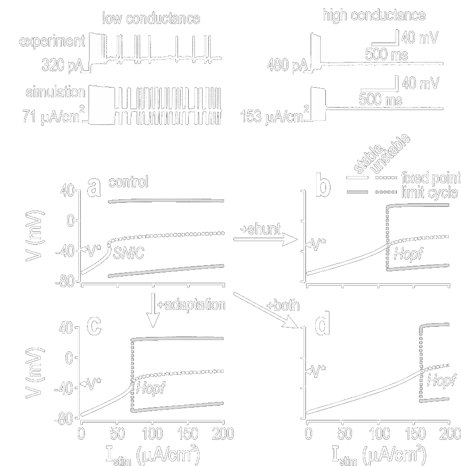
Using this model, one can readily demonstrate the following dynamical phenomena:

Using XPPAUT and choosing relevant bifurcation parameters show the transition from SNIC to Hopf bifurcation and how each of them affect the F-I characteristic of the CA1 pyramidal neuron (Response property) : Effectively you will be replicating the first few figures of the paper. Suggestion is that you start with the Iext vs V and move from there.
Show how the background noise affects the transition in dynamics. Does more noise favour one dynamical system (SNIC vs Hopf) vs other ?
Dissect out the role of adaptation vs shunting . Are there any other bifurcation parameters that can be used to understand the behaviour of the system ?
Replicate these neurons in your favourite neuron simulator. This will be convenient for making the F-I curve for different system configurations. Although in principle XPPAUT can also be used for the same.
Make a network of these neurons in your favorite neuron simulator. For the inhibitory neurons (PV basket cell or O-LM) you can use simple integrate and fire type neurons with synapse characteristics matching the CA1. Compare the two configurations (SNIC vs Hopf) in both high inhibitory and low inhibitory settings.
Visualize V and w nullclines and observe how changing gM, beta_w (or any other parameter you think is important ) changes the nullcline geometry and (oscillatory) approach to equilibrium.
Show that a particular class supports subthreshold oscillation more than the other.
Compare the coding properties of integrator and resonator neurons by stimulating them with constant currents, pulses, ramps, chirps, noisy currents, and Poisson synaptic trains, and quantify differences in spike latency, phase locking, coincidence detection, temporal precision, vector strength, and transfer function.

Suggestion : Look at chapter - 7 - Neuronal Excitability Izhkevich for more clarity about class 1 and class 2 behavior.

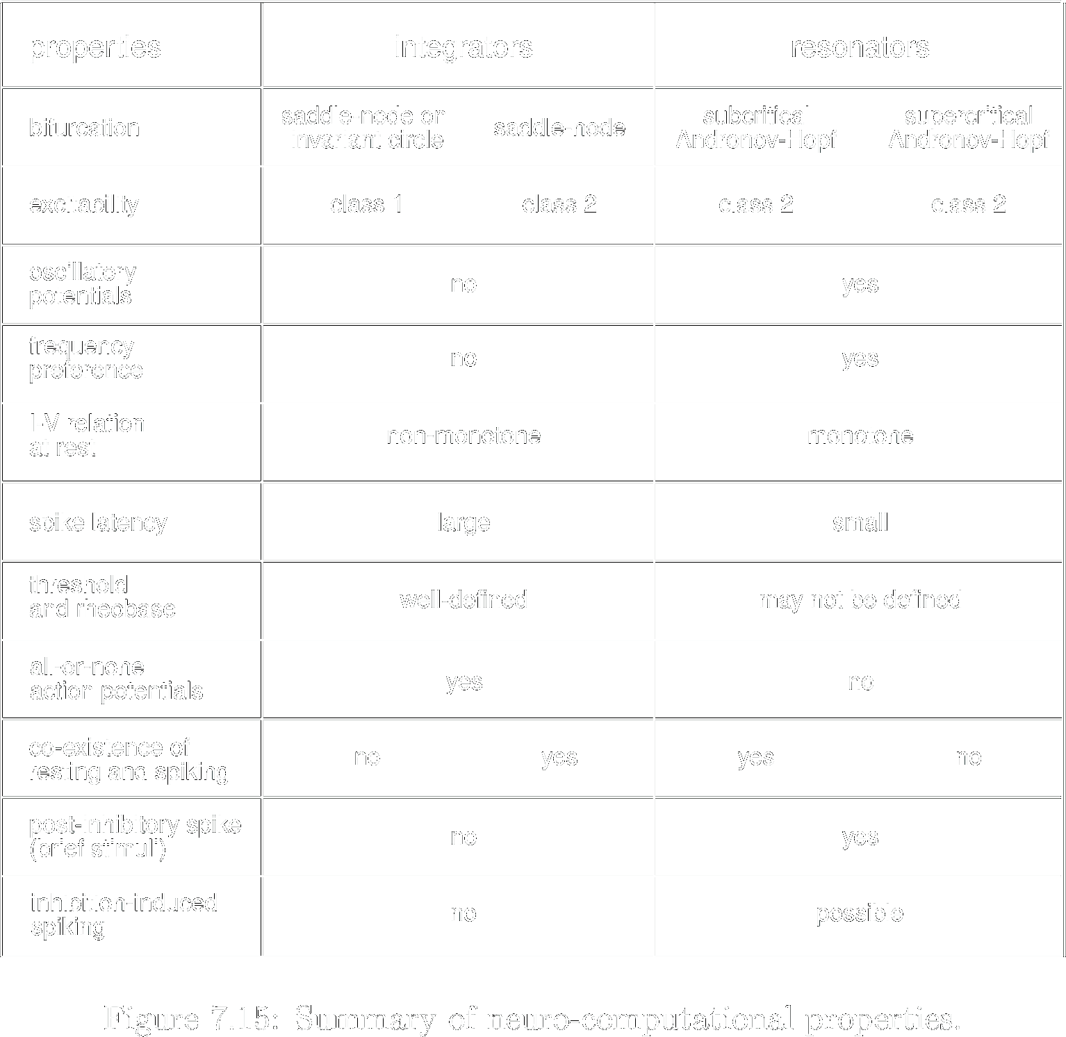
Reference : Izhekevich’s Book

You can do many more things with this model. Abovementioned suggestions are just characterizations of the model. Some interesting broad questions to ask might be :

A. Does one configuration support a particular kind of computation vs other ? For example : Are resonator neurons better coincidence detectors?

B. How does the excitability class influence network synchronization? What kind of computation can synchronization promote ?

C. Can a heterogeneous population containing both SNIC and Hopf neurons outperform homogeneous populations?

D. Is there an optimal adaptation time constant for hippocampal computation? Can the network dynamically switch computational modes during behavior?

E. Construct a network (Hint : Link) consisting of excitatory pyramidal neurons together with inhibitory PV basket cells (or O-LM interneurons), compare network dynamics when the pyramidal cells operate in the SNIC versus Hopf regime under both low and high inhibition, and quantify synchrony, population firing rate, theta/gamma power, pairwise correlations, and phase locking to determine whether resonator neurons synchronize more readily. Hint : You do not necessarily have to replicate inhibitory neuronal dynamics, you can use spike trains and simple inhibitory synapse with some reasonable time constants.

Project 9: Small world network of Excitable neurons show self sustained activity (Roxin, Reike and Solla 2004)

Persistent activity arising from network bistability is widely considered a candidate mechanism for working memory. Although numerous cortical network models have explored this phenomenon, the role of network architecture—particularly connectivity heterogeneity and long-range excitatory interactions—remains relatively underexplored. Investigating how these structural features influence network dynamics may help clarify the principles governing stable memory representations in cortical circuits. These self sustained activity can also be seen in models studying epilepsy and bursting in pre-botZ complexes. The group of Sara A. Solla showed that at low coupling (or connection probability) the network can show failure to propagate or succeed. (paper)

Consider an array of N integrate-and-fire (IF) neurons as described in the paper :

Characterize how each parameter (tauD, gsyn, etc.) affects the overall firing pattern.
Construct a small world network of these neurons in such a way that :

a) Local connections are modeled as nearest-neighbors coupling (as in the paper) (Wij = 1 if i and j are neighbors) . You can use brian2, NEURON or any of your favourite simulators.

b) Setup a long range connection from randomly adding a pn fraction of unidirectional connections.

c) Calculate some network properties like clustering coefficient, closeness, betweenness and correlate it with the firing property of the network. Does it intuitively tell you anything ?

d) Make a network of 1000 neurons with different values of I, gsyn tau_membrane and tau_d . Confirm that for some value of these parameters, you start seeing persistent activity with some failure and successes. (Iext = 0.85, gsyn = 0.2,tau_m = 10 , tau_d = 1 ). The activity vanishes if connectivity or coupling is reduced ? Check that as well.

e) Design an algorithm to check whether the activity persists or not (failure vs success) and how long the activity persisted with a single injection of input.

f) For different p from 0 to 1 (for instance, p = 0.1 ∗ k, k = 1, … , 10), average over 2000 realizations to calculate the probability of persistent activity. Plot the complementary probability of failure versus p, for N = 250, 1500, 1000, 2000 and comment the results. Observe that the probability of failure is an increasing function of p with increasing steepness as the size N of the system increases.
Calculate clustering coefficient, closeness centrality, and betweenness centrality and correlate them with network firing properties.
Construct networks of ~1000 neurons and identify regimes that support persistent activity.
Design an algorithm to classify simulations into failure versus success and measure persistence duration.
Reproduce the probability-of-failure analysis for different network sizes and rewiring probabilities.

You can do many more things with this model. The above suggestions are merely characterizations of the model.

Some broader questions that may be interesting to investigate:

A. Can the network show input-dependent durations of persistent activity?

B. Can you find out if the duration of persistent activity is a reliable quantity to store memory ?

C. What should be the connectivity of a network to give a somewhat reliable number of successes ? Do areas in the brain implicated in Working memory show connectivity close to this ?

D. Do brain regions implicated in working memory exhibit similar connectivity statistics?

Project 10: Functional balanced networks with synaptic plasticity (Sadeh et al 2015)

Github Repository

During the development of the visual cortex, synaptic connectivity is non-specific that later becomes functional and selective via several processes including synaptic pruning. One specific example of this is synaptic connections of orientation-selective neurons in the rodent visual cortex. However in the rodents the distribution of orientation selective neurons is different from primates. More specifically in rodents, in contrast, such spatial orientation maps do not exist, and neurons of different specificities are mixed in a salt-and-pepper fashion..Sadeh Rotter and Clopath ( Sadeh et al ) show that feature-specific connectivity can arise in realistic neocortical networks of excitatory and inhibitory neurons . They also show that such networks with plastic recurrent synapses can, through visual experience, develop specific connectivity. However there is an E-I balance that is maintained before and after training.

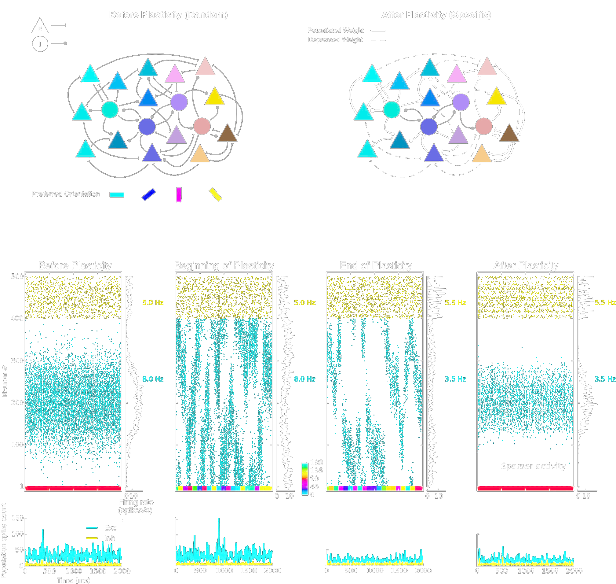
Using this model, one can readily demonstrate the following phenomena:

You can create this model in Brian2, NEURON, or any of your favorite neuron simulators, or use the model provided by the authors in the GitHub repository. Calculate total excitatory versus total inhibitory current and examine how it evolves before and after plasticity.
Start from random connectivity. Train for 40 training batches and plot the weight matrix before and after training (and also (Wf - Wi)). Verify that neurons with similar preferred orientations develop stronger E→E connections.
For every neuron, calculate the tuning curve and determine its preferred orientation. You can also calculate the mean OSI (Orientation Selectivity Index) before and after training. Does synaptic plasticity sharpen tuning after training? Does learning make coding more sparse?
Change the number of training batches (repeated training blocks) and the number of different stimuli (number of stimuli with different orientations in each batch). Figure out how these variables affect learning.
Change the trial time and repeat the analysis in (4). Are the results intuitive?
Change the timescales of plasticity and repeat the analysis in (4). Does learning make coding more sparse?
Isolate one presynaptic and one postsynaptic cell and construct the plasticity kernel. Is potentiation symmetric? Does the rule generate bidirectional connectivity?
Systematically vary E→E synaptic strength and connectivity. Calculate selectivity, OSI, and sparsity. Is there a critical connectivity density required for learning?

You can do many more things with this model. The above suggestions are merely characterizations of the model.

A. Small-World vs Random Connectivity: Replace the random E→E network with Erdős-Rényi, Small-world, and Scale-free architectures and compare learning speed and final specificity. This is a particularly interesting extension project.

B. Population Dynamics (Dimensionality Reduction): Construct population firing rate vectors and perform PCA. Compare PCA trajectories before and after training. Does learning compress stimulus representations?

C. Weight Distribution Dynamics: Calculate the evolution of the synaptic weight distribution over training. Why does a bimodal distribution emerge? You can also use information-theoretic approaches to explain this phenomenon.

Project 11: Activity state of random networks with dynamic synapses

Networks with static synapses have been extensively studied. Much less is known about networks in which E and I neurons are connected with dynamic (facilitatory/depressing) synapses.

Set-up a network of integrate and fire neurons (at least 4K exc and 1K inh.). We use a simple neuron model as we are interested in the effect of synapse dynamics.
Connect the neurons randomly or in a spatial manner (your choice) There are four types of synapses in your model. E→ E, E→ I, I→ E, I→ I. Each could be a facilitatory or depressing type. Making EE synapses facilitatory could be risky as it could destabilize the network when operated at high frequencies. What is the right combination of the synapses that keeps the network stable and also allows it to exhibit different types of dynamical states. You can start by introducing dynamic synapses in EI and IE synapses.
Compare the states with a network in which synapses are static. Are there differences? Do we need to define new descriptors to capture the dynamics of a network in which synapses are dynamic?

Please refer to:

Uziel A, Markram H. t 2000: Synchrony generation in recurrent networks with frequency- dependent synapses (https://doi.org/10.1523/jneurosci.20-01-j0003.2000)

And some other papers of Misha Tsodyks could give you a good start.

Project 12: Local connectivity and directional anisotropy can lead to the emergence of spatiotemporal sequences in spiking neuronal networks

Brian Code

Paper Link

Many of the networks/regions in the brain encode relevant information in a spatiotemporal code. But the understanding of mechanisms behind how these patterns might emerge, remains incomplete. Sebastian Spreizer, Ad, and Arvind proposed a more biologically plausible connectivity rule which gives rise to spatiotemporal activity in a network of Leaky integrate and Fire neurons. What they suggest is that a directional anisotropy in the connectivity, in addition to local connectivity rules, can achieve this.

You can do the following things in this framework :

Show that a purely inhibitory network produces a significantly different spatiotemporal pattern than networks with excitation-inhibition of perlin networks. (as in paper). Investigate the effect of synaptic weights and time scales (synaptic taus) on generation of these patterns.
Analyse the power spectra of different network configurations. How is it affected by the strength of synaptic input ?
Test that the asymmetry and coupling determines the velocity of spatiotemporal activity patterns that emerge. You can make a two-dimensional plot for Extent of asymmetry on one axis and coupling (extent of local connections) on other and plot vmax. What does it tell you about the system ?
Change the extent of the perlin noise. Change it systematically and figure out how spatial patterns emerge with different extent of asymmetry of the network.
Give input to a small set of local neighbouring neurons. How the spatiotemporal patterns emerge in different connectivity schemes.

Many more interesting things can be done with this model. For starters, does leak affect the emergence of spatiotemporal patterns ? Or is a reset mechanism enough for this in a perlin network? Next thing, is there a phase locking to the global oscillation of the network ? Authors also suggest that asymmetric modulation by neuromodulation like dopamine can also help in creating such a pattern.

Project 13: Spontaneous calcium oscillations in Astrocytes and IP3-dependent Calcium Dynamics in Astrocytes

(Laventovich and Hemkin 2008, Handy et al 2017)

Github Repository Paper 1

Github Repository Paper 2

Tiina Manninen Replication in Python Paper 1

Astrocytes, once considered passive support cells, are now widely accepted as active participants in neural signaling. Activity-dependent increases in astrocytic intracellular Ca²⁺ trigger the release of gliotransmitters such as glutamate and ATP, which modulate neuronal activity. This has led to the tripartite synapse concept, where pre- and postsynaptic neurons and astrocytes communicate bidirectionally. Astrocyte–neuron interactions influence synaptic plasticity, including long-term depression (LTD), and are implicated in neurological disorders such as epilepsy. In many of these cases where astrocytes are seen to interact with their environment, a change in the concentration or oscillatory behavior of the astrocyte’s [Ca2+] cyt appears to be an integral step in the process. Experiments show that while the changes in the astrocyte’s oscillatory Ca2+ behavior is often found to be a result of external stimulation, these oscillations can also be formed spontaneously. These spontaneous oscillations are ubiquitous (and reported in both in situ and several parts of the brain. Laventovich and Hemkin were able to investigate key mechanistic steps of this process using a mathematical model of astrocyte’s Ca2+ oscillations and were able to replicate various experimental phenomena related to this process. Nearly a decade later, Handy et al. extended this line of work by asking a different question. Rather than simply explaining why oscillations occur, they investigated why astrocytes display such a rich diversity of calcium responses. Their model incorporates IP3 receptor dynamics, SERCA pumps, PMCA pumps, ER leak currents and store-operated calcium (SOC) channels into a more detailed nonlinear dynamical system. A central conclusion of their work is that the different experimentally observed calcium response types are largely determined by the underlying bifurcation structure of the system rather than by arbitrary parameter choices. Unlike neuronal models, where injected current is typically used as the bifurcation parameter, here the physiologically meaningful control parameter is the intracellular IP3 concentration itself. This makes astrocytes an excellent system for studying nonlinear dynamics in a directly biological context. Together these two papers provide an excellent introduction to nonlinear biochemical dynamics. The first paper explains how oscillations emerge, whereas the second explains how those oscillations are organized in parameter space. The models are sufficiently simple to explore using XPPAUT while still capturing many experimentally observed calcium dynamics.

Using this model, one can readily demonstrate the following phenomena:

Simulate spontaneous calcium oscillations in the Lavrentovich and Hemkin model. Show that oscillations arise without any externally applied stimulus and investigate how changing the basal calcium influx parameter (Vin) changes the behaviour of the system. Identify the range of parameters for which spontaneous oscillations exist and compare the simulated oscillation period with that reported in the paper. 2.Investigate how astrocytic calcium dynamics change when : -SERCA pump activity is reduced, -IP3 receptor conductance is reduced, calcium influx across the membrane is altered. Explain mechanistically why each manipulation changes the oscillatory behaviour.

Effect of plasma membrane calcium influx .
IP3 degradation effects. Explain mechanistically why each manipulation changes the oscillatory behaviour. Relate each manipulation to the corresponding biological experiment.

Using the Handy model, reproduce the four experimentally observed calcium response classes: Single Peak, Multipeak , Plateau and Long-lasting response types. Determine how changes in intracellular IP3 move the system between these response types.
Draw the bifurcation diagram of the Handy model using intracellular IP3 as the continuation parameter. Identify stable equilibrium, unstable equilibrium, stable limit cycles,Hopf bifurcations (try to explain it if you can from a reduced form of equations), and relate each calcium response to its location within the bifurcation diagram.

You can do many more things with this model. The above suggestions are merely characterizations of the model.

A. Frequency encoding versus amplitude encoding: One long-standing question in calcium signalling is whether information is encoded primarily through oscillation frequency, oscillation amplitude, oscillation duration or combinations of all three. Stimulate the astrocyte using different IP3 waveforms. (pulses,ramps,sinusoidal inputs,noisy inputs) and determine which quantities change most reliably.

B. Choose another additional parameter as a bifurcation parameter and redraw the bifurcation diagram for it. Which parameters merely shift the bifurcation, and which fundamentally alter the qualitative dynamics?

C. Instead of varying a single parameter, construct two-parameter bifurcation diagrams for Ex: IP3 - SERCA. Identify the regions of oscillations, steady states and bistability etc.

D. The Lavrentovich model briefly demonstrates that changing only a few parameters can generate period-adding behaviour and even chaotic oscillations. Reproduce these results and investigate the route to chaos. Does the system undergo period doubling, period adding or some other transition? Also for this model : Plot nullclines and trajectories and identify fast and slow variables.

E. Real astrocytes exhibit considerable cell-to-cell variability. Perform a sensitivity analysis by varying multiple parameters simultaneously. Which mechanisms produce robust oscillations? Which parameters require tight biological regulation? Are spontaneous oscillations merely biological noise, or do they carry functional information? What advantages do astrocytes acquire by operating near the onset of oscillatory behaviour?