Week 2 Project Ideas

Tip

These are just suggested project ideas. You are free to come up with your own. You can also use last week’s unused projects.

Project 1: Spike Packet Transfer

Recurrently connected networks are excellent models to study the propagation of synchronous neural signals. Here we will construct a similar network and study the propagation of synchronisation.

Construction:

Construct spiking neuronal models. These can be leaky integrate-and-fire models or conductance-based models. Importance is given to the spiking characteristics of the models. The models receive a background noise, which can lead to spontaneous spiking. This is the modelled synaptic noise. The neurons are connected in a feed-forward manner, with the excitatory and inhibitory connections modelled as alpha functions of opposite signs.

Initialization:

The neurons are excited in the first layer by a spike volley. A volley is characterised by (i) the number of spikes, ain, and (ii) the temporal dispersion of the spikes, σin.

Progression:

As time progresses, in each layer of the network, one can observe the size and dispersion of the volley. As such, one can trace the values a and σ across the different layers as time progresses. This gives the state space of the spiking.

Find the dynamics of the state space. Find the different fixed points in the system. How do the different hyperparameters, like the time constant of the neurons, the size of the network, the noise parameters, etc., affect the fixed points? Plot the bifurcation plots for the system.

You may refer to this study: Stable propagation of synchronous spiking in cortical neural networks (https://doi.org/10.1038/990101).

Project 2: Simple model of central pattern generators

You have already looked at one simple network of central pattern generators of STG. You can now recreate a network model of a CPG of your choice. It can be conductance based, integrate and fire neurons, Izhikevich models etc. Preferably one with at least some excitatory synapses. Use this model to answer the following:

1. What is the source of oscillation? Is it driven by the pacemaker neuron or does it arise from the network connectivity?

2. Are there neurons that oscillate in the absence of synaptic inputs? If yes, what parameters allow them to do so? Can you now use these to make others in the network oscillatory?

3. If you were a neuromodulator and your goal was to change the rhythm of the network, how would you do it? Is it sufficient to change the rhythm of the pacemaker circuit or do you also have to change the synaptic weights? Check out this review to see how neuromodulatory action can modulate CPG activity: Neuromodulation of circuits with variable parameters: single neurons and small circuits reveal principles of state-dependent and robust neuromodulation ([https://doi.org/10.1146/annurev-neuro-071013-013958])

Bonus: Construct a “Parameterscape” for your CPG as is done in Multiple Mechanisms Switch an Electrically Coupled, Synaptically Inhibited Neuron between Competing Rhythmic Oscillators (https://doi.org/10.1016/j.neuron.2013.01.016).

Below are some models you can use for reference:

1. Tritonia swim network

   a. (Peter Getting, 1989): https://modeldb.science/93326

   b. (Calin-Jagemann, 2007): https://modeldb.science/93325

2. STG network (Eve marder and colleagues):

   a. https://modeldb.science/3511

   b. https://modeldb.science/93321

   c. https://modeldb.science/224998] [https://pubmed.ncbi.nlm.nih.gov/15558066/

For the more ambitious (and with better computation power), you can go one step further and see how changing the network affects movement. Below are two models for your reference:

1. Tadpole spinal cord network: https://modeldb.science/267146

2. Zebrafish spinal cord network: https://github.com/Bui-lab/Code

Project 3: DSI and continuous attractor network

Make a continuous attractor network with neurons exhibiting spike rate adaptation. Why can’t the network stably store the memory for a long time? Implement a slow activity-dependent local disinhibition for example cannabinoid-dependent depolarization-induced suppression of inhibition (DSI) to make the bump more stable. Replicate the figures produced by https://doi.org/10.1093/cercor/bhm103

Project 4: Intrinsically bursting HVC-RA

Jin et al 2007: Intrinsic bursting enhances the robustness of a neural network model of sequence generation by avian brain area HVC (https://doi.org/10.1007/s10827-007-0032-z), describes a model of a network of songbird HVC neurons that can generate sequences. This model relies on the idea that individual HVC-RA neurons are capable of intrinsically bursting.

1. Reproduce this model.

2. Now, can you vary parameters in the HVC-RA neurons and see what is the regime under which these neurons burst intrinsically?

Project 5: Effect of dendritic morphology and ion channel distribution in single neuron models

• First try to reproduce the results for inward (terminal->soma) and outward (soma->terminal) input sequence from [Rall, W. (1964). Theoretical significance of dendritic trees for neuronal input-output relations. In R. F. Reiss (Ed.), Neural Theory and Modeling (pp. 73-97). Stanford Univ. Press. https://doi.org/10.7551/mitpress/6743.003.0015 ]

• Then create a simple passive neuronal arbor with symmetric branching that gets thinner and thinner with distance from soma and attach synaptic inputs at various locations and observe the effect of activation of those synapses.

• Finally add various ion channels to all compartments, vary the conductance densities based on distance from the dendrite terminals, and explore the effect of synaptic inputs.

• Pick a few interesting neuronal morphologies from neuromorpho.org and do the same experiment. What are the effects of input at different parts of the dendritic arbor?

Project 6: Local feedback via dendrites

Create a neuron A with a large dendritic arbor (you can pick some existing model) and create two single compartmental neurons B and C and connect them reciprocally to A. Compare the outcomes when:

(1) the synapses B-A, A-B, C-A, and A-C are all to and from the same compartment of A with

(2) the scenario where they are on different branches of A.

Start with passive models and then gradually add K+, Ca2+ and Na+ channels and see the results. What happens when you make the A-B and A-C synapses inhibitory?

Project 7: Effect of dendritic morphology and ion channel distribution in single neuron models

• First try to reproduce the results for inward (terminal->soma) and outward (soma->terminal) input sequence from [Rall, W. (1964). Theoretical significance of dendritic trees for neuronal input-output relations. In R. F. Reiss (Ed.), Neural Theory and Modeling (pp. 73-97). Stanford Univ. Press.]
• Then create a simple passive neuronal arbor with symmetric branching that gets thinner and thinner with distance from soma and attach synaptic inputs at various locations and observe the effect of activation of those synapses
• Finally add various ion channels to all compartments, vary the conductance densities based on distance from the dendrite terminals, and explore the effect of synaptic inputs
• Pick a few interesting neuronal morphologies from neuromorpho.org and do the same experiment. What are the effects of input at different parts of the dendritic arbor?

Project 8: Local feedback via dendrites

Create a neuron A with a large dendritic arbor (you can pick some existing model) and create two single compartmental neurons B and C and connect them reciprocally to A. Compare the outcomes when (1) the synapses B-A, A-B, C-A, and A-C are all to and from the same compartment of A with (2) the scenario where they are on different branches of A. Start with passive models and then gradually add K+, Ca2+ and Na+ channels and see the results. What happens when you make the A-B and A-C synapses inhibitory?

Project 9: Graded Persistent Activity

Eye position:

The saccadic eye movement is an interesting model to study how specialised neural circuits can implement important physiological functions. The angular eye position instils a change in the firing frequency of the pre-motor neuron in the prepositus hypoglossi and the medial vestibular nucleus. The change in the firing frequency is mediated by a transient pulse of input from command neurons and persists for the duration of the fixation. Here we model this network.

Model the network as described in: Stability of the memory of eye position in a recurrent network of conductance-based model neurons. This is a hand-tuned model of the goldfish integrator. As the model is sensitive to the exact values of the synaptic parameters, you’ll have to pay careful attention to how you implement it. It can be done in NEURON, but the units of the different quantities will have to be carefully adjusted.

1. Comment about the physiology of the integrator. What aspects of the model impart its characteristic function?

2. Find the dynamics of the different neurons in the network. Use linear and non-linear dimensionality reduction techniques to establish the scheme of the attractor in play in the network.

3. How can you make the network more robust to parameter changes?

Project 10: Grid Cells and Reinforcement Learning

Between model-free and model-based RL, there is a compromise called the Successor Representation. Stachenfeld, Gershman and Botvinick (2017) found a surprising relation between the Successor Representation and so-called grid cell firing patterns in the enthorinal cortex. Recreate their Supplementary Figures S7 and S8. Extra credit: Try some other environment shapes. Can you reproduce any of the figures from the main paper? https://www.nature.com/articles/nn.4650

Project 12: A spiking version of the SimpleQLearner:

Using Brian, create two populations of neurons. Make pairs of neurons from the same population excite each other, but neurons from different populations inhibit each other. That way, you can have the two populations “compete” with each other so that only one population is active at a time. The “action” is simply defined as the population that is active. Stimulate the network with some background activity. Let the synaptic strength from “background” to each population code for the respective Q-value. What should the synaptic learning rule look like for the updates to correspond to the RL update rule from the tutorial? Can you justify that rule from a biological point of view? What spiking neuron parameters might correspond to the RL parameters α and β?

Extra credit 1 (if there is time): Add more than one state by adding multiple groups of “background activity” and make it so that each group of background activity is active when that state is active (“one-hot coding”). Can you make the network big enough to solve a full 5x5 gridworld problem? (Might be computationally expensive…)

Extra credit 2: Instead of updating the synapses directly when there is reward, create a separate population of neurons that code for the RPE (“dopamine neurons”) and use their firing rates to update the synapses.

Project 11: MCell

Astrocytic processes, especially perisynaptic astrocytic processes (PAPs), are thin (~100–300 nm diameter) and highly dynamic. These microdomains:

• Enwrap synapses

• Are rich in IP₃ receptors (IP₃Rs) on internal endoplasmic reticulum membranes

• Exhibit localized spontaneous Ca²⁺ signals called blips (single-channel events) and puffs (multi-channel events)

Experimental challenge: Due to their tiny size, these compartments are below the resolution of standard fluorescence microscopy, making it hard to determine:

• Molecular mechanisms

• Spatial organization

• Origin of spontaneous calcium signals

Particle-based spatial stochastic simulation is ideal for capturing:

• Spatial localization of receptors and signaling molecules

• Stochastic fluctuations in small volumes

• Colocalization-driven feedback mechanisms

This is where MCell comes in — a platform for realistic 3D, particle-based simulations of cell signalling at nanoscales.

Objectives

1. Replicate a spatial, stochastic model of spontaneous Ca²⁺ signaling via IP3Rs in fine astrocytic processes.

2. Quantify how IP₃R clustering (η) and calcium source colocalization radius (Rγ) affect:

   • Open probability of IP3 receptors

   • Amount of calcium in the cytosol

   • Proportion of blips vs puffs

All parameters and model details are provided in the paper below:.

Reference paper:

https://journals.plos.org/ploscompbiol/article?id=10.1371/journal.pcbi.1006795

“Simulation of calcium signaling in fine astrocytic processes: Effect of spatial properties on spontaneous activity”

Audrey Denizot, Misa Arizono, U. Valentin Nägerl, Hédi Soula, Hugues Berry

Project 12: MCell

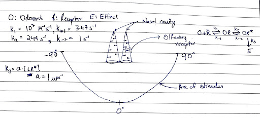
What is that smell? Where is it coming from? We have often found ourselves pondering these questions, regardless of the source of that smell. Interestingly, we are not alone in this inquiry; all complex organisms can ask the same. The olfactory system is arguably the oldest sensory system and is present across these organisms, allowing them to identify the source of an odorant by adjusting their nasal cavities or antennae and comparing the incoming signals.

In this project, you will design two identical conical nasal cavities using CellBlender and simulate the response of olfactory receptors to a diffusing odorant. By studying the dynamics of the receptors in the nasal cavity, can you determine the direction or angle of the odorant’s source? If so, please explain the underlying principle that enables the detection of the source’s direction or angle from the nasal cavity. Additionally, comment on the resolution of your system. Feel free to draw your own conclusions as well.

Feel free to play around with the rate constants.

You may use the following papers for further reference:

1. https://bpspubs.onlinelibrary.wiley.com/doi/pdfdirect/10.1002/prp2.311
2. https://pubs.acs.org/doi/10.1021/acs.jpcb.7b00486

Project 13: From spiking neurons to population dynamics — example on Wilson-Cowan model

Objective:

This project explores how the collective behavior of neural populations emerges from the interactions of individual spiking neurons. Using probabilistic methods inspired by Bressloff [1] and Benayoun et al. [2], the Wilson-Cowan equations [3,4] are derived from microscopic spiking dynamics. The analysis of this mean-field model explains key phenomena like bistability and oscillations in neural activity.

1. Mean-Field Approximation:

Let’s consider a network of stochastic binary neurons (0: quiescent state and 1: active state). Each neuron spiking (jump from 0 to 1) probability depends on its inputs from the other excitatory and inhibitory neurons. Considering the dynamics of the proportion of active neurons when the number of neurons tends to infinity, one can derive a mean field model which is nothing else than the famous WIlson-Cowan model.

2. Emergent Phenomena:

Analysing the limit system with dynamical system theory, one can find parameters generating interesting dynamics such as bistability and oscillations.

3. Numerical Exploration:

Simulations of the Wilson-Cowan model and its microscopic version enables one to visualize these phenomena, mapping out parameter regimes where bistability or oscillations occur.

4. Discussion:

What are the strengths and limitations of the mean-field approach? Consider when it breaks down (e.g., in small or highly correlated networks) and possible extensions to include noise or spatial structure.

Outcome:

The project highlights the interplay between theory (mean-field approximations) and phenomena (bistability, oscillations), offering intuition for how simplified models can capture complex neural behavior.

References:

[1] Bressloff, P. C. Metastable states and quasicycles in a stochastic Wilson-Cowan model of neuronal population dynamics. Physical Review E 82, 051903 (2010).

[2] Benayoun, M., Cowan, J. D., van Drongelen, W. & Wallace, E. Avalanches in a Stochastic Model of Spiking Neurons. PLoS Computational Biology 6, e1000846 (2010).

[3] Wilson, H. R. & Cowan, J. D. Excitatory and Inhibitory Interactions in Localized Populations of Model Neurons. Biophysical Journal 12, 1—24 (1972).

[4] Wilson, H. R. & Cowan, J. D. A mathematical theory of the functional dynamics of cortical and thalamic nervous tissue. Kybernetik 13, 55—80 (1973).

Project 14: Bring me a Neuronal morphology that can….! :

This project is concerned with characteristic ‘passive’ properties of neurons and how they affect neuronal signal processing. We have the following properties that we can study:

i) The electric properties: Rm, Ra, Cm. ii) The morphology of the neuronal sections: Diameter, Length (of both the soma and the dendrites) iii) The topology of the neuron–arborization with multiple dendrites: makes neurons with at least 2 dendrites. iv) Distribution of synapses: synapses on same dendrites vs multiple dendrites.

This is a simple project to implement, so the analysis has to be very rigorous. One way to go about this would be to define a repertoire of different neurons and try the same experiments with different neurons.

1. Model a biophysically realistic model of neuron. Have two copies of the neuron – one with only passive leak currents and one with active ion channels. Make sure you have enough complex neuron models such all the properties above can be studied. Make sure to use appropriate compartmentalisation.
2. Impinge the neurons with different types of currents – constant current, white noise, and Poisson. Comment about the differences observed when the properties mentioned above are changed.
3. Distribute the synapses on the dendrites: either distribute the synapses on the same dendrite at different distances from the soma, or distribute them at different dendrites at the same distance from the soma.
4. Activate some synapses – how does the EPSP travel in the dendrites of various characteristics? Stimulate all simultaneously, or with Poisson statistics. What are the differences observed?
5. Observe and comment about the temporal and spatial summation of the stimuli.
6. Perform the same analyses with active ion channels. How do the various characteristics change?
7. Add white noise to the models. How does this change the temporal and spatial summation?

Analyse the results with physiological significance and constraints in mind. Your analyses should rigorously analyse the effect of the changes in different properties in phenomena like dendritic integration (both temporally and spatially) and attenuation (for complex and simpler arborization). You are welcome to include complexity in model and study other relevant phenomena. But your analyses should reflect on its physiological importance.

Project 15: Electrophysiology and Neural Coding

In this project, we will analyse the coding properties of a neuron and how they vary with different neuronal characteristics.

Make a conductance-based model of a neuron with active conductance. You can include any number of ion channels in the model as you like, or even model a neuron with empirically observed ion channels and corresponding conductance. The only requirement is that it should fire action potentials.

1. Identify the default firing mode of the neuron (classify it into a class I, class II or class III neuron).

2. Modulate the different ion channel properties of channels in the neuron and find out which channels change the firing mode of the neuron.

3. Find out the channel properties corresponding to the three classes of neurons. As such, create a repertoire of class I, class II and class III neurons starting from the base model.

4. Why does the firing mode of the neurons change with the different properties? Show in context of different ion channel currents.

5. Find out the temporal summation characteristics of the signals impinged on the neuron and how they vary for the three classes.

6. Find out the Spike Triggered Average (STA) for the three classes of neurons. Comment on the Input-Output properties of the neuron.

7. Create a set of similar classes of neurons and impinge them with a variety of synchronous and asynchronous inputs.

8. Repeat 6 with various types and amounts of noise. Analyze the effects of correlation in inputs and noise on the correlation of the output.

Comment on what role the various classes of neurons can play in a network.

Bonus: If you have not already, introduce HCN, NaP, SK and CaT type currents in the neuronal model and analyse the effects of the ion channels on the coding characteristics.

For reference, please refer to the excellent review: Impact of Neuronal Properties on Network Coding: Roles of Spike Initiation Dynamics and Robust Synchrony Transfer (http://dx.doi.org/10.1016/j.neuron.2013.05.030)